本文主要介绍函数 gwr_multiscale() 的用法。
基本用法
我们以示例数据 LondonHP 为例,展示函数 gwr_multiscale() 的用法。 假设我们以 PURCHASE 为因变量,FLOORSZ, PROF 和 UNEMPLOY 为自变量,可以使用下面的方式构建多尺度 GWR 模型。
data(LondonHP)
m1 <- gwr_multiscale(
 formula = PURCHASE ~ FLOORSZ + UNEMPLOY + PROF,
 data = LondonHP
)
m1
Multiscale Geographically Weighted Regression Model
===================================================
  Formula: PURCHASE ~ FLOORSZ + UNEMPLOY + PROF
     Data: LondonHP


Parameter-specified Weighting Configuration
-------------------------------------------
                 bw   unit type   kernel longlat p theta optim_bw criterion
Intercept  3758.992 Meters Null gaussian   FALSE 2     0     TRUE       AIC
FLOORSZ    1684.743 Meters Null gaussian   FALSE 2     0     TRUE       AIC
UNEMPLOY  45226.177 Meters Null gaussian   FALSE 2     0     TRUE       AIC
PROF      13000.959 Meters Null gaussian   FALSE 2     0     TRUE       AIC
             threshold centered
Intercept 1.000000e-05    FALSE
FLOORSZ   1.000000e-05     TRUE
UNEMPLOY  1.000000e-05     TRUE
PROF      1.000000e-05     TRUE


Summary of Coefficient Estimates
--------------------------------
 Coefficient        Min.     1st Qu.      Median     3rd Qu.        Max.
   Intercept  125497.191  132762.279  150831.667  168818.165  190110.170
     FLOORSZ    -184.067     997.289    1506.309    1970.043    3027.671
    UNEMPLOY  310326.670  315433.209  318711.539  320575.312  325930.524
        PROF  222076.169  236767.029  248433.345  258565.543  274402.517


Diagnostic Information
----------------------
  RSS: 230041770180
  ENP: 69.67341
  EDF: 246.3266
   R2: 0.8715428
R2adj: 0.8350606
 AICc: 7486.598
这里展示的是在不进一步设置变量的情况下调用函数,函数默认以如下配置设置算法
- 无初始带宽
- 非可变带宽
- 高斯核函数
- 非地理坐标系
- 欧氏距离度量
- 中心化非截距变量
- 根据 AIC 值优选带宽
- 带宽优选收敛阈值为 \(10^{-5}\)
大多数情况下,这样设置可以保证算法能够运行。如需进一步定制参数,请参考加权配置
该函数返回一个 gwrmultiscalem 的对象,通过控制台输出信息,我们可以得到 调用的表达式、数据、带宽、核函数、系数估计值的统计、诊断信息。 同样,也支持使用 coef() fitted() residuals() 等函数获取信息。
  Intercept   FLOORSZ UNEMPLOY     PROF
0  136571.4 1125.6123 317951.9 222076.2
1  136399.8 1088.7621 317908.4 222413.4
2  134523.3 1198.3076 318342.1 223189.3
3  134101.9 1167.6316 318365.7 223632.4
4  135117.1 1070.7761 318056.3 223445.3
5  136170.9  972.5949 317036.1 223865.2
[1] 340891.9 335865.2 329410.1 363434.9 367997.6 347934.2
[1] -183891.9 -222365.2 -247660.1 -213434.9 -177997.6 -187984.2
此外,与旧版 GWmodel 包类似,gwrmultiscalem 对象中提供了一个 $SDF 变量保存了系数估计值等一系列局部结果。
Simple feature collection with 6 features and 6 fields
Geometry type: POINT
Dimension:     XY
Bounding box:  xmin: 531900 ymin: 159400 xmax: 535700 ymax: 161700
CRS:           NA
  Intercept   FLOORSZ UNEMPLOY     PROF     yhat  residual
0  136571.4 1125.6123 317951.9 222076.2 340891.9 -183891.9
1  136399.8 1088.7621 317908.4 222413.4 335865.2 -222365.2
2  134523.3 1198.3076 318342.1 223189.3 329410.1 -247660.1
3  134101.9 1167.6316 318365.7 223632.4 363434.9 -213434.9
4  135117.1 1070.7761 318056.3 223445.3 367997.6 -177997.6
5  136170.9  972.5949 317036.1 223865.2 347934.2 -187984.2
               geometry
0 POINT (533200 159400)
1 POINT (533300 159700)
2 POINT (532000 159800)
3 POINT (531900 160100)
4 POINT (532800 160300)
5 POINT (535700 161700)
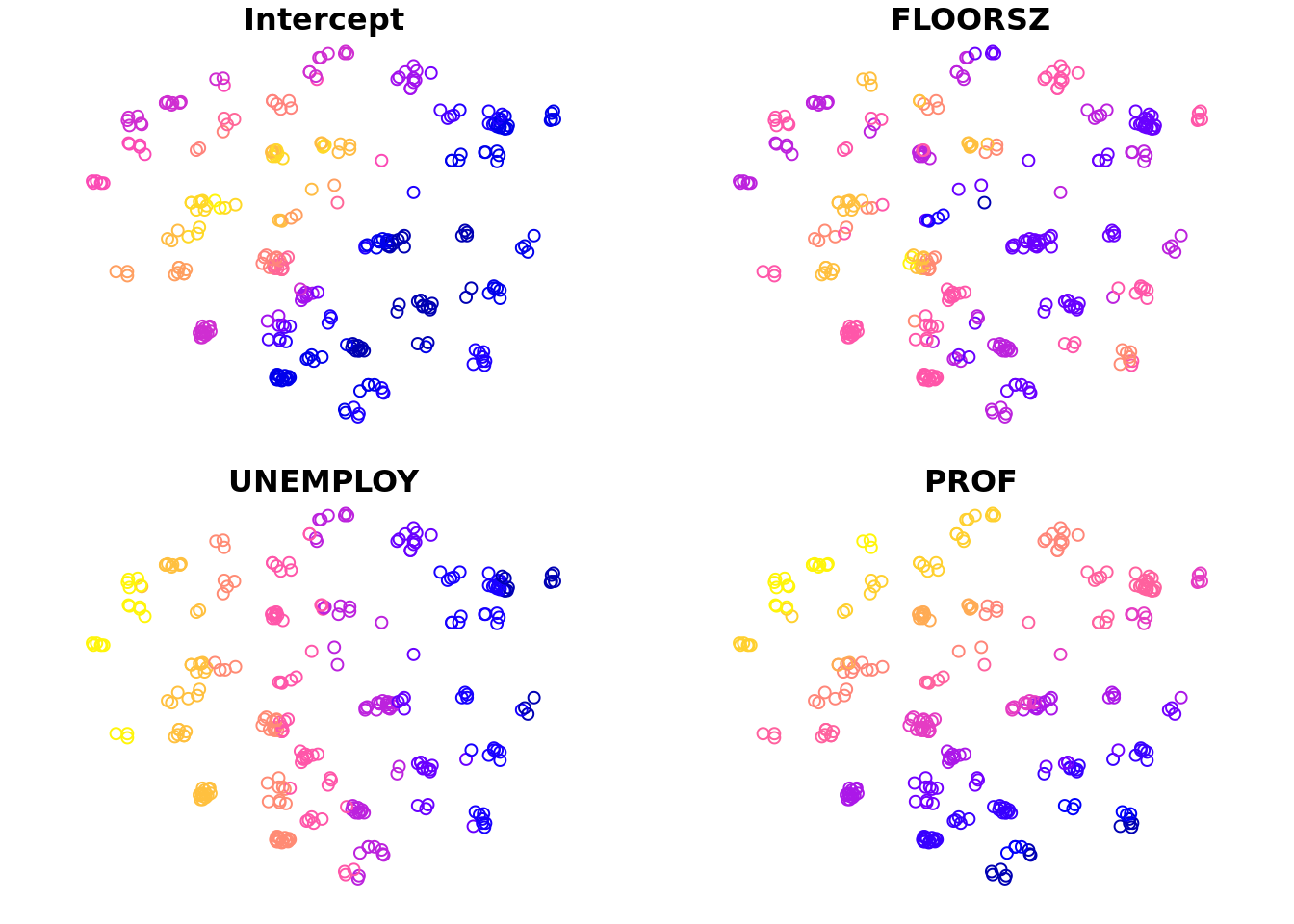
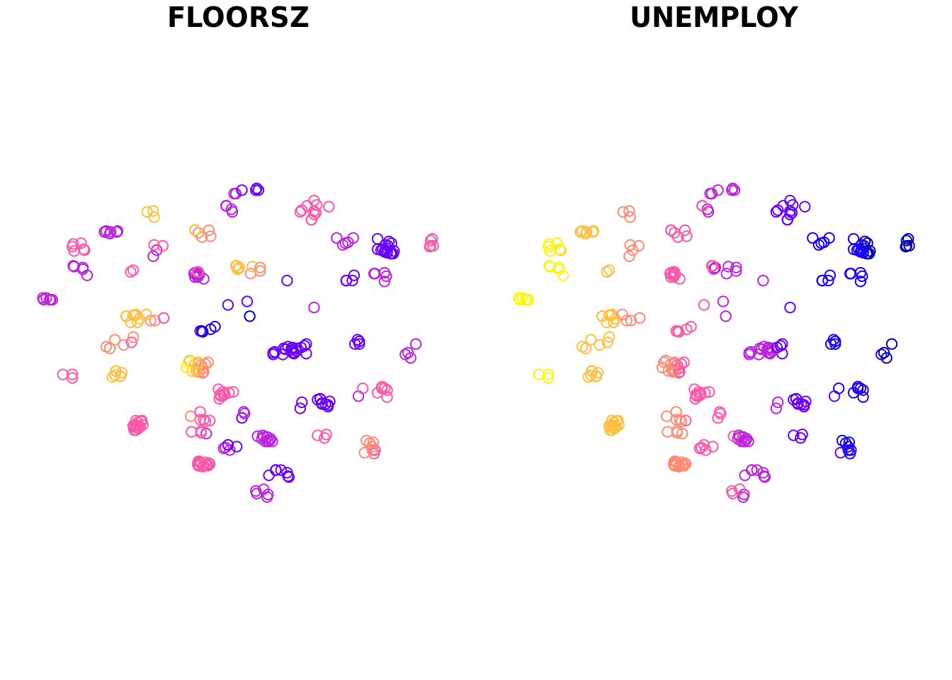
使用该变量,可以进行专题制图。除此之外,改包还提供了一个 plot() 函数,通过输入 gwrmultiscalem 对象,可以快速查看回归系数。
plot(m1, columns = c("FLOORSZ", "UNEMPLOY"))
如果指定了 columns 参数,则仅绘制第二个参数列出的系数,否则绘制所有回归系数。
加权配置
多尺度加权配置选项
包中定义了一个 MGWRConfig 的 S4 类型,用于提供多尺度加权配置的设置。 该类型的对象包含以下几个成员:
bw |
Numeric |
带宽值。 |
adaptive |
Logical |
是否为可变带宽。 |
kernel |
Character |
核函数名称。 |
longlat |
Logical |
是否为经纬度坐标。 |
p |
Numeric |
Minkowski 距离次数。 |
theta |
Numeric |
Minkowski 距离旋转角度。 |
centered |
Logical |
是否中心化变量。 |
optim_bw |
Character |
是否优选带宽以及带宽优选指标。如果值是 "no" 则不再进行带宽优选。否则根据指定的指标值进行优选。 |
optim_threshold |
numeric |
带宽优选阈值。 |
使用函数 mgwr_config() 可以直接构造一个对象。
mgwr_config(36, TRUE, "bisquare", optim_bw = "AIC")
An object of class "MGWRConfig"
Slot "bw":
[1] 36

Slot "adaptive":
[1] TRUE

Slot "kernel":
[1] "bisquare"

Slot "longlat":
[1] FALSE

Slot "p":
[1] 2

Slot "theta":
[1] 0

Slot "centered":
[1] TRUE

Slot "optim_bw":
[1] "AIC"

Slot "optim_threshold":
[1] 1e-05
该类型的对象也支持使用 rep() 函数复制,但支持持 times 参数。
rep(mgwr_config(36, TRUE, "bisquare", optim_bw = "AIC"), 2)
[[1]]
An object of class "MGWRConfig"
Slot "bw":
[1] 36

Slot "adaptive":
[1] TRUE

Slot "kernel":
[1] "bisquare"

Slot "longlat":
[1] FALSE

Slot "p":
[1] 2

Slot "theta":
[1] 0

Slot "centered":
[1] TRUE

Slot "optim_bw":
[1] "AIC"

Slot "optim_threshold":
[1] 1e-05


[[2]]
An object of class "MGWRConfig"
Slot "bw":
[1] 36

Slot "adaptive":
[1] TRUE

Slot "kernel":
[1] "bisquare"

Slot "longlat":
[1] FALSE

Slot "p":
[1] 2

Slot "theta":
[1] 0

Slot "centered":
[1] TRUE

Slot "optim_bw":
[1] "AIC"

Slot "optim_threshold":
[1] 1e-05
使用 MGWRConfig 进行参数配置
函数 gwr_multiscale() 既可以统一设置加权配置项,也可以分别设置加权配置项。
统一设置
如果要给所有变量统一设置加权配置项,可以传入只包含一个 MGWRConfig 类型对象的列表。 例如,将所有变量的带宽类型设置为可变带宽,核函数设置为 Bi-square 核函数。
m2 <- gwr_multiscale(
 formula = PURCHASE ~ FLOORSZ + UNEMPLOY + PROF,
 data = LondonHP,
 config = list(mgwr_config(adaptive = TRUE, kernel = "bisquare"))
)
m2
Multiscale Geographically Weighted Regression Model
===================================================
  Formula: PURCHASE ~ FLOORSZ + UNEMPLOY + PROF
     Data: LondonHP


Parameter-specified Weighting Configuration
-------------------------------------------
           bw unit type   kernel longlat p theta optim_bw criterion
Intercept  92   NN Null bisquare   FALSE 2     0     TRUE       AIC
FLOORSZ    19   NN Null bisquare   FALSE 2     0     TRUE       AIC
UNEMPLOY   51   NN Null bisquare   FALSE 2     0     TRUE       AIC
PROF      157   NN Null bisquare   FALSE 2     0     TRUE       AIC
             threshold centered
Intercept 1.000000e-05    FALSE
FLOORSZ   1.000000e-05     TRUE
UNEMPLOY  1.000000e-05     TRUE
PROF      1.000000e-05     TRUE


Summary of Coefficient Estimates
--------------------------------
 Coefficient         Min.     1st Qu.      Median     3rd Qu.         Max.
   Intercept   128027.588  134315.206  147425.383  168778.168   185788.635
     FLOORSZ      -71.171     999.976    1480.660    1938.071     3736.606
    UNEMPLOY  -537304.673  108123.294  611883.562  902220.559  2303154.999
        PROF   163822.997  221234.648  246805.452  300170.581   348794.459


Diagnostic Information
----------------------
  RSS: 221062803902
  ENP: 68.95713
  EDF: 247.0429
   R2: 0.8765567
R2adj: 0.8419599
 AICc: 7474.897
由于 centered 选项默认为 TRUE,因此函数在运行时, 会自动将截距对应的加权配置项中的 centered 变量设置为 FALSE 以避免可能存在的问题。
同样的,也可以使用 rep 函数,但是要确保传入正确的 times 变量的值。
m2 <- gwr_multiscale(
 formula = PURCHASE ~ FLOORSZ + UNEMPLOY + PROF,
 data = LondonHP,
 config = rep(mgwr_config(adaptive = TRUE, kernel = "bisquare"), times = 4)
)
分别设置
如果分别设置加权配置项,则需要传入包含与自变量(如果有截距也包括截距)相同数量的 MGWRConfig 对象的列表。
m3 <- gwr_multiscale(
 formula = PURCHASE ~ FLOORSZ + UNEMPLOY + PROF,
 data = LondonHP,
 config = list(mgwr_config(bw = 92, adaptive = TRUE, kernel = "bisquare"),
               mgwr_config(bw = 19, adaptive = TRUE, kernel = "bisquare"),
               mgwr_config(bw = 51, adaptive = TRUE, kernel = "bisquare"),
               mgwr_config(bw = 157, adaptive = TRUE, kernel = "bisquare"))
)
m3
Multiscale Geographically Weighted Regression Model
===================================================
  Formula: PURCHASE ~ FLOORSZ + UNEMPLOY + PROF
     Data: LondonHP


Parameter-specified Weighting Configuration
-------------------------------------------
           bw unit    type   kernel longlat p theta optim_bw criterion
Intercept  92   NN Initial bisquare   FALSE 2     0     TRUE       AIC
FLOORSZ    19   NN Initial bisquare   FALSE 2     0     TRUE       AIC
UNEMPLOY   51   NN Initial bisquare   FALSE 2     0     TRUE       AIC
PROF      157   NN Initial bisquare   FALSE 2     0     TRUE       AIC
             threshold centered
Intercept 1.000000e-05    FALSE
FLOORSZ   1.000000e-05     TRUE
UNEMPLOY  1.000000e-05     TRUE
PROF      1.000000e-05     TRUE


Summary of Coefficient Estimates
--------------------------------
 Coefficient         Min.     1st Qu.      Median     3rd Qu.         Max.
   Intercept   128027.588  134315.206  147425.383  168778.168   185788.635
     FLOORSZ      -71.171     999.976    1480.660    1938.071     3736.606
    UNEMPLOY  -537304.673  108123.294  611883.562  902220.559  2303154.999
        PROF   163822.997  221234.648  246805.452  300170.581   348794.459


Diagnostic Information
----------------------
  RSS: 221062803902
  ENP: 68.95713
  EDF: 247.0429
   R2: 0.8765567
R2adj: 0.8419599
 AICc: 7474.897
这样就可以通过使用 c() rep() 等函数的组合灵活设置每个变量的配置项。