In this page we introduce the usage of function gwr_basic().
library(sf)
#> Linking to GEOS 3.7.1, GDAL 2.4.0, PROJ 5.2.0; sf_use_s2() is TRUE
library(GWmodel3)
#>
#> Attaching package: 'GWmodel3'
#> The following object is masked from 'package:stats':
#>
#>     step
Model Calibration
We use the LondonHP data as an example to demonstrate how to use function gwr_basic(). Assume that the PURCHASE is the dependent variable, while FLOORSZ and UNEMPLOY are independent varaibles. We can build a GWR model through the folloing way.
data(LondonHP)
m1 <- gwr_basic(
    formula = PURCHASE ~ FLOORSZ + UNEMPLOY + PROF,
    data = LondonHP,
    bw = 64,
    adaptive = TRUE
)
m1
#> Geographically Weighted Regression Model
#> ========================================
#>   Formula: PURCHASE ~ FLOORSZ + UNEMPLOY + PROF
#>      Data: LondonHP
#>    Kernel: gaussian
#> Bandwidth: 64 (Nearest Neighbours)
#>
#>
#> Summary of Coefficient Estimates
#> --------------------------------
#>  Coefficient         Min.      1st Qu.       Median      3rd Qu.        Max.
#>    Intercept  -198642.679  -182675.271  -165665.781  -134650.946  -93550.292
#>      FLOORSZ     1189.823     1309.140     1399.934     1668.918    1840.670
#>     UNEMPLOY   311994.460   531503.077   663356.786   735359.196  932328.652
#>         PROF   243840.288   319870.143   355123.025   378312.489  429390.257
#>
#>
#> Diagnostic Information
#> ----------------------
#>   RSS: 4.56323e+11
#>   ENP: 14.12809
#>   EDF: 301.8719
#>    R2: 0.7451855
#> R2adj: 0.7332201
#>   AIC: 7571.953
#>  AICc: 7585.417
Compared with GWmodel, the usage is changed in the following ways:
- The function is renamed to
gwr_basicto avoid conflicts with the old version. - The function no longer support the
regression.pointsargument. To predict at new locations, please use thepredict()function. - The OLS part is no longer shown in outputs of the return value. Users can call
lm()function with specified arguments.
This function return a gwrm object. Through the outputs in console, we can get infromation of fomula, data, kernel, bandwidth, coefficient estimates, and diagnostics. Besides, it is supported to get more infromation via coef() fitted() residuals().
head(coef(m1))
#>   Intercept  FLOORSZ UNEMPLOY     PROF
#> 0 -124453.6 1287.804 528674.5 295482.3
#> 1 -122812.0 1282.712 520067.3 293203.2
#> 2 -122487.0 1281.506 530303.5 291236.4
#> 3 -121768.6 1278.788 527744.3 290153.6
#> 4 -122064.9 1278.969 520144.8 291861.3
#> 5 -101753.7 1234.532 396245.5 263582.0
head(fitted(m1))
#> [1] 135011.1 132297.2 117858.7 157436.0 173050.9 157071.0
head(residuals(m1))
#> [1]  21988.936 -18797.233 -36108.677  -7436.005  16949.120   2879.028
In addition, like GWmodel, gwrm objects provide a $SDF variable which contains coefficient estimates and other sample-wise results.
head(m1$SDF)
#> Simple feature collection with 6 features and 14 fields
#> Geometry type: POINT
#> Dimension:     XY
#> Bounding box:  xmin: 531900 ymin: 159400 xmax: 535700 ymax: 161700
#> CRS:           NA
#>   Intercept  FLOORSZ UNEMPLOY     PROF     yhat   residual Intercept.SE
#> 0 -124453.6 1287.804 528674.5 295482.3 135011.1  21988.936      5839925
#> 1 -122812.0 1282.712 520067.3 293203.2 132297.2 -18797.233      5873318
#> 2 -122487.0 1281.506 530303.5 291236.4 117858.7 -36108.677      5962947
#> 3 -121768.6 1278.788 527744.3 290153.6 157436.0  -7436.005      5990687
#> 4 -122064.9 1278.969 520144.8 291861.3 173050.9  16949.120      5928749
#> 5 -101753.7 1234.532 396245.5 263582.0 157071.0   2879.028      6126740
#>   FLOORSZ.SE UNEMPLOY.SE PROF.SE Intercept.TV  FLOORSZ.TV UNEMPLOY.TV
#> 0   351842.1    14680113 7170057  -0.02131082 0.003660175  0.03601297
#> 1   353135.2    14735103 7214234  -0.02091015 0.003632355  0.03529444
#> 2   356231.7    14939953 7324666  -0.02054135 0.003597394  0.03549566
#> 3   357162.0    14994222 7360524  -0.02032632 0.003580416  0.03519651
#> 4   354868.2    14840291 7285505  -0.02058864 0.003604066  0.03504950
#> 5   363613.1    15108910 7586125  -0.01660813 0.003395180  0.02622595
#>      PROF.TV              geometry
#> 0 0.04121060 POINT (533200 159400)
#> 1 0.04064233 POINT (533300 159700)
#> 2 0.03976104 POINT (532000 159800)
#> 3 0.03942024 POINT (531900 160100)
#> 4 0.04006054 POINT (532800 160300)
#> 5 0.03474527 POINT (535700 161700)
We can create maps with this variable. There is a plot() function provided to preview coefficient estimates easily.
plot(m1)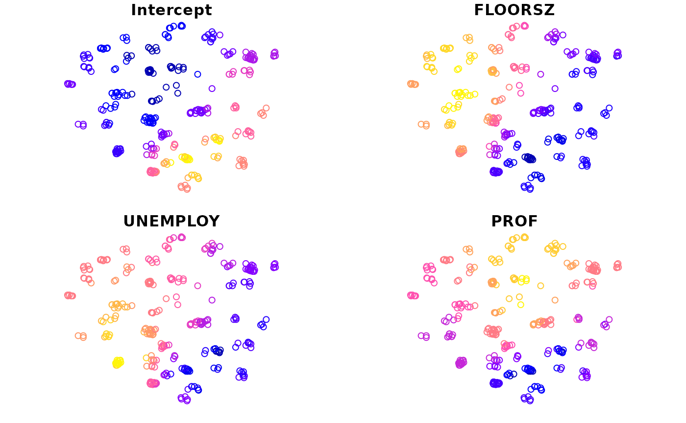
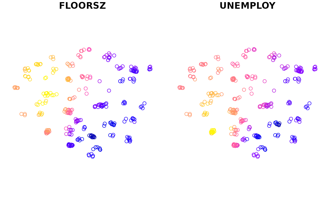
If the second argument is omitted, all coefficient estimates will be mapped by default. Otherwise, only specified variables will be mapped.
Bandwidth Optimization
We can call the function in the following way when we want the function to get an optimized bandwidth instead.
data(LondonHP)
m <- gwr_basic(
    formula = PURCHASE ~ FLOORSZ + UNEMPLOY,
    data = LondonHP,
    bw = "AIC",
    adaptive = TRUE
)
message("Bandwidth:", m$args$bw)
#> Bandwidth:20
The method for optimizing bandwidth is specified through strings "AIC" or "CV". Besides, when argument bw is missing or set to non-numeric values, this function select an optimized bandwidth according to AIC values.
To obtain the value of optimized bandwidth, use the variable $args$bw of the returned object, or read it from console output.
Model Selection
In this package, there is a generic function called step(). We we apply it to gwrm objects, it can select variables, just like the stepAIC() in MASS.
m2 <- gwr_basic(
    PURCHASE ~ FLOORSZ + UNEMPLOY + PROF + BATH2 + BEDS2 + GARAGE1 +
        TYPEDETCH + TPSEMIDTCH + TYPETRRD + TYPEBNGLW + BLDPWW1 +
        BLDPOSTW + BLD60S + BLD70S + BLD80S + CENTHEAT,
    LondonHP, "AIC", TRUE
)
m2 <- step(m2, criterion = "AIC", threshold = 10, bw = Inf, optim_bw = "AIC")
m2
#> Geographically Weighted Regression Model
#> ========================================
#>   Formula: PURCHASE ~ FLOORSZ + PROF + UNEMPLOY
#>      Data: LondonHP
#>    Kernel: gaussian
#> Bandwidth: 20 (Nearest Neighbours) (Optimized accroding to AIC)
#>
#>
#> Summary of Coefficient Estimates
#> --------------------------------
#>  Coefficient         Min.      1st Qu.       Median      3rd Qu.         Max.
#>    Intercept  -283403.492  -202450.678  -146322.221   -26250.365    75680.532
#>      FLOORSZ      908.249     1095.711     1411.257     1864.155     2482.376
#>         PROF   -16595.354   143221.798   303155.382   379563.029   480351.828
#>     UNEMPLOY  -982984.259    -5935.799   575766.002  1029212.413  1780751.157
#>
#>
#> Diagnostic Information
#> ----------------------
#>   RSS: 348701748965
#>   ENP: 40.26956
#>   EDF: 275.7304
#>    R2: 0.8052821
#> R2adj: 0.7767406
#>   AIC: 7506.818
#>  AICc: 7546.36
There are two arguments: bw and optim_bw. This is the way to use them:
- When
bwis missing or isNA, then the bandwidth recorded ingwrmobject is used. - When
bwis numeric, its value is used in model optimization. The value ofoptim_bwdetermined whether optimize bandwidth again before finally calibrate it.- When
optim_bwis"no", skip the bandwidth optimization process. - When
optim_bwis"AIC"or"CV", optimize bandwidth according to the corresponding criterion.
- When
- When
bwis non-numeric, useInfas the bandwidth value to optimize bandwidth. And use the criterion specified byoptim_bwto optimize bandwidth. Whenoptim_bwis"no", use the AIC criterion by default.
It seems to be complicated, but it is easy to use. On most occassions, set paramters like the example above.
The returned object after model selection contains a $step variable, in which there are all model combinations and corresponding criterions. There are three functions to visualize it.
step_view_circle(m2$step, main = "Circle View")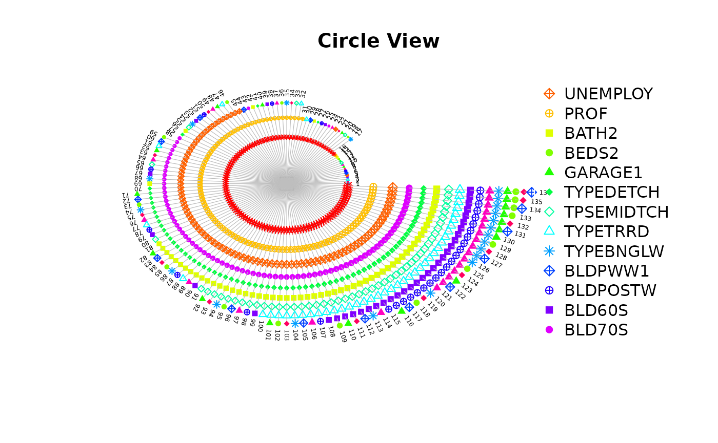
step_view_value(m2$step, main = "AIC Value")
step_view_diff(m2$step, main = "Diff of AIC")
We can also use the universal plot() function which will make some modification to layouts.
plot(m2$step, main = "Circle View") # step_view_circle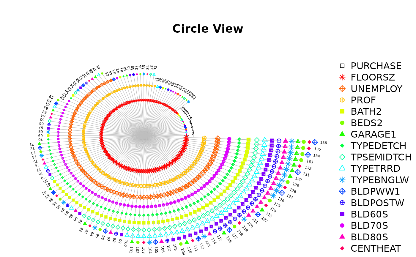
plot(m2$step, main = "AIC Value", view = "value") # step_view_value
plot(m2$step, main = "Diff of AIC", view = "diff") # step_view_diff
If further modification is required, use other arguments supported by plot().
Predict
Based on the current model, GWR can predict coefficient values at any position. We can use predict() function.
predict(m2, LondonHP)
#> Simple feature collection with 316 features and 6 fields
#> Geometry type: POINT
#> Dimension:     XY
#> Bounding box:  xmin: 507400 ymin: 159400 xmax: 552300 ymax: 194900
#> CRS:           NA
#> First 10 features:
#>    Intercept   FLOORSZ      PROF   UNEMPLOY     yhat   residual
#> 0 -23859.461 1107.8783 143091.28  -68568.68 127499.2  29500.837
#> 1 -19273.643 1099.6911 137317.02 -105774.02 125164.0 -11664.024
#> 2 -22341.033 1101.6762 139576.72  -78733.42 112173.3 -30423.269
#> 3 -16587.207 1091.7319 131959.65 -127715.69 145741.0   4259.021
#> 4  -4548.212 1071.6907 118805.43 -236130.77 158572.5  31427.480
#> 5  36721.681 1025.9964  69162.51 -574801.77 158491.4   1458.602
#> 6  41385.027 1015.8069  64587.38 -621772.02 139520.0  10475.019
#> 7  41586.375  980.2804  72971.83 -702105.05 206972.8  32977.160
#> 8  57682.066  985.6583  47493.74 -778290.44 158200.9  -5200.854
#> 9  71221.072  928.7546  43974.22 -982984.26 310010.7 -60060.651
#>                geometry
#> 0 POINT (533200 159400)
#> 1 POINT (533300 159700)
#> 2 POINT (532000 159800)
#> 3 POINT (531900 160100)
#> 4 POINT (532800 160300)
#> 5 POINT (535700 161700)
#> 6 POINT (535600 161800)
#> 7 POINT (533400 161900)
#> 8 POINT (535500 162200)
#> 9 POINT (534200 162500)
The result varies depends on the second argument:
- When it is a
sforsfcobject, the function will return asforsfcobject including the orignal geometries. - When it is a two-column matrix or
data.frame, the function will return adata.frameobject without geometries.
Besides, when the second argument is a sf or sfc object, the returned value varies depends on its attributes:
- When it does not contains all of independent variables, only coefficient estimates will be returned.
- When it only contains all of independent variables, coefficient and dependent variable estimates will be returned.
- When it contains all of independent variables and the dependent variable, coefficient estimates, dependent variable estimates and residuals will be returned.
Then we can get different results for different demands.