Multiscale GWR • GWmodel3

In this page we mainly introduce the usage of gwr_multiscale().

library(sf)
#> Linking to GEOS 3.7.1, GDAL 2.4.0, PROJ 5.2.0; sf_use_s2() is TRUE
library(GWmodel3)
#> 
#> Attaching package: 'GWmodel3'
#> The following object is masked from 'package:stats':
#> 
#>     step

Basics

Let us set the data LondonHP as an example, and show how to use gwr_multiscale(). Assume that the PURCHASE is the dependent variable, while FLOORSZ, PROF and UNEMPLOY are independent variable, we can calibrate a multiscale GWR model with the following code.

data(LondonHP)
m1 <- gwr_multiscale(
  formula = PURCHASE ~ FLOORSZ + UNEMPLOY + PROF,
  data = LondonHP
)
m1
#> Multiscale Geographically Weighted Regression Model
#> ===================================================
#>   Formula: PURCHASE ~ FLOORSZ + UNEMPLOY + PROF
#>      Data: LondonHP
#> 
#> 
#> Parameter-specified Weighting Configuration
#> -------------------------------------------
#>                  bw   unit type   kernel longlat p theta optim_bw criterion
#> Intercept  3758.992 Meters Null gaussian   FALSE 2     0     TRUE       AIC
#> FLOORSZ    1684.743 Meters Null gaussian   FALSE 2     0     TRUE       AIC
#> UNEMPLOY  45226.177 Meters Null gaussian   FALSE 2     0     TRUE       AIC
#> PROF      13000.959 Meters Null gaussian   FALSE 2     0     TRUE       AIC
#>              threshold centered
#> Intercept 1.000000e-05    FALSE
#> FLOORSZ   1.000000e-05     TRUE
#> UNEMPLOY  1.000000e-05     TRUE
#> PROF      1.000000e-05     TRUE
#> 
#> 
#> Summary of Coefficient Estimates
#> --------------------------------
#>  Coefficient        Min.     1st Qu.      Median     3rd Qu.        Max. 
#>    Intercept  125497.191  132762.279  150831.667  168818.165  190110.170 
#>      FLOORSZ    -184.067     997.289    1506.309    1970.043    3027.671 
#>     UNEMPLOY  310326.670  315433.209  318711.539  320575.312  325930.524 
#>         PROF  222076.169  236767.029  248433.345  258565.543  274402.517 
#> 
#> 
#> Diagnostic Information
#> ----------------------
#>   RSS: 230041770180
#>   ENP: 69.67341
#>   EDF: 246.3266
#>    R2: 0.8715428
#> R2adj: 0.8350606
#>  AICc: 7486.598

Here no additional arguments are set, so the function will apply the follwing configurations:

No initial value for bandwidth.
Fixed bandwdith.
Guassian kernel function.
Projective coordinate reference system.
Euclidean distance metrics.
Centrolized non-intercept independent variables.
AIC criterion for bandwidth optimization.
A threshold of $10^{-5}$ for bandwidth optimization.

On most situations, these configurations can ensure the algorithm works. To further specify arguments, please turn to Weighting configurations.

This function returns a object of class name gwrmultiscalem. Through the outputs in console, we can get infromation of fomula, data, kernel, bandwidth, coefficient estimates, and diagnostics. Besides, it is supported to get more infromation via coef() fitted() residuals().

head(coef(m1))
#>   Intercept   FLOORSZ UNEMPLOY     PROF
#> 0  136571.4 1125.6123 317951.9 222076.2
#> 1  136399.8 1088.7621 317908.4 222413.4
#> 2  134523.3 1198.3076 318342.1 223189.3
#> 3  134101.9 1167.6316 318365.7 223632.4
#> 4  135117.1 1070.7761 318056.3 223445.3
#> 5  136170.9  972.5949 317036.1 223865.2
head(fitted(m1))
#> [1] 340891.9 335865.2 329410.1 363434.9 367997.6 347934.2
head(residuals(m1))
#> [1] -183891.9 -222365.2 -247660.1 -213434.9 -177997.6 -187984.2

In addition, like the old version, gwrmultiscalem objects provide a $SDF variable which contains coefficient estimates and other sample-wise results.

head(m1$SDF)
#> Simple feature collection with 6 features and 6 fields
#> Geometry type: POINT
#> Dimension:     XY
#> Bounding box:  xmin: 531900 ymin: 159400 xmax: 535700 ymax: 161700
#> CRS:           NA
#>   Intercept   FLOORSZ UNEMPLOY     PROF     yhat  residual
#> 0  136571.4 1125.6123 317951.9 222076.2 340891.9 -183891.9
#> 1  136399.8 1088.7621 317908.4 222413.4 335865.2 -222365.2
#> 2  134523.3 1198.3076 318342.1 223189.3 329410.1 -247660.1
#> 3  134101.9 1167.6316 318365.7 223632.4 363434.9 -213434.9
#> 4  135117.1 1070.7761 318056.3 223445.3 367997.6 -177997.6
#> 5  136170.9  972.5949 317036.1 223865.2 347934.2 -187984.2
#>                geometry
#> 0 POINT (533200 159400)
#> 1 POINT (533300 159700)
#> 2 POINT (532000 159800)
#> 3 POINT (531900 160100)
#> 4 POINT (532800 160300)
#> 5 POINT (535700 161700)

We can create maps with this variable. There is a plot() function provided to preview coefficient estimates easily.

plot(m1)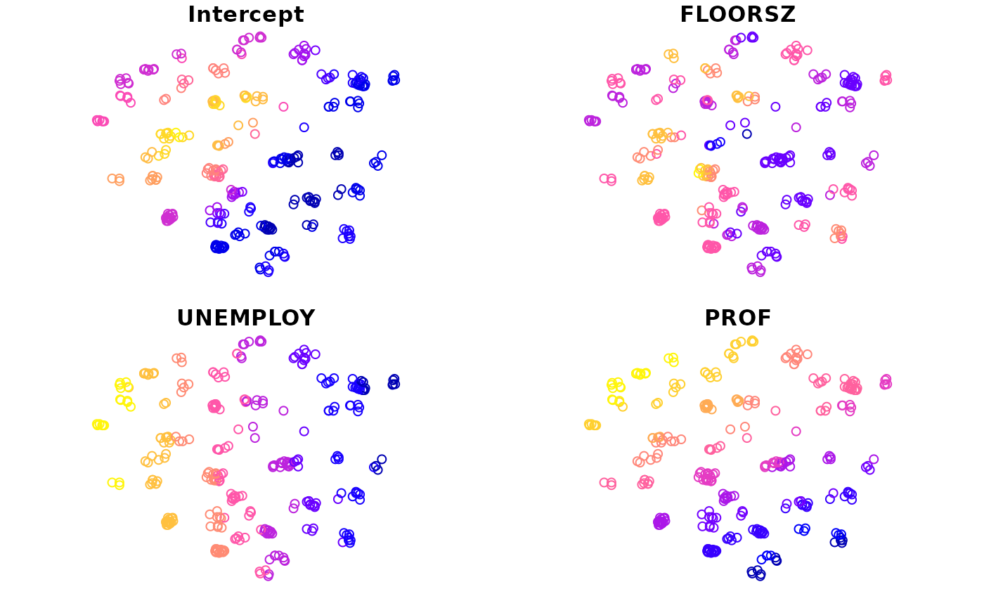

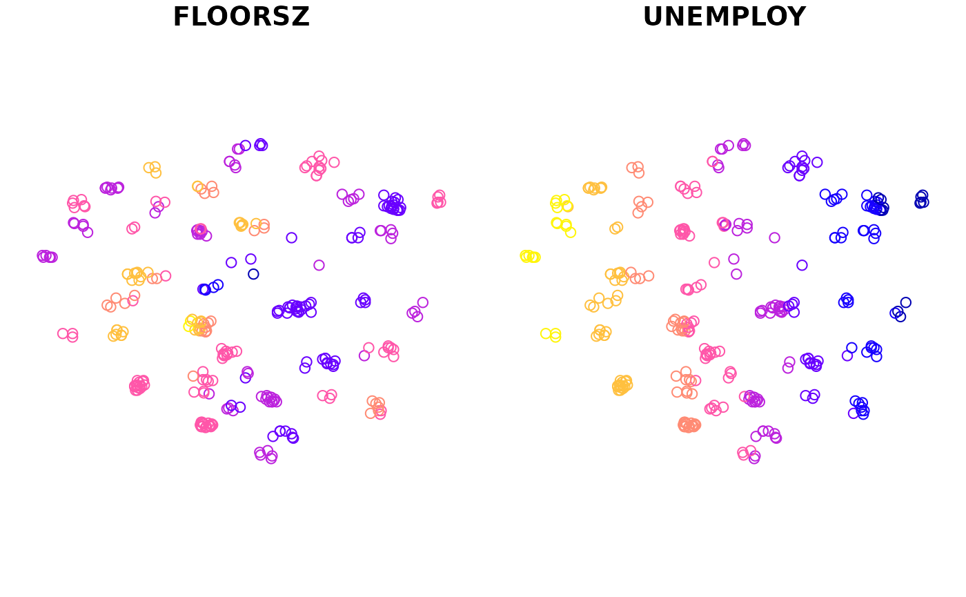
plot(m1, columns = c("FLOORSZ", "UNEMPLOY"))

If the second argument is omitted, all coefficient estimates will be mapped by default. Otherwise, only specified variables will be mapped.

Weighting configurations

S4 class for multiscale weighting configrations

This package provides a S4 class named MGWRConfig, which is used to set multiscale weighting configurations. This class contains the following slots:

Slot	Type	Descirption
`bw`	Numeric	Bandwidth.
`adaptive`	Logical	Whether the bandwidth is adaptive
`kernel`	Character	Name of kernel function.
`longlat`	Logical	Whether coordinates are longitudes and latitudes.
`p`	Numeric	The power of Minkowski distance metrics.
`theta`	Numeric	The angle of Minkowski distance metrics.
`centered`	Logical	Whether to centrolize variables.
`optim_bw`	Character	Whether to optimize bandwidth and the criterion’s name if yes. Use `"no"` to disable bandwidth optimization; otherwise, set the bandwidth criterion’s name here.
`optim_threshold`	numeric	THe threshold of bandwidth optimization.

We can use the function mgwr_config() to create an object.

mgwr_config(36, TRUE, "bisquare", optim_bw = "AIC")
#> An object of class "MGWRConfig"
#> Slot "bw":
#> [1] 36
#> 
#> Slot "adaptive":
#> [1] TRUE
#> 
#> Slot "kernel":
#> [1] "bisquare"
#> 
#> Slot "longlat":
#> [1] FALSE
#> 
#> Slot "p":
#> [1] 2
#> 
#> Slot "theta":
#> [1] 0
#> 
#> Slot "centered":
#> [1] TRUE
#> 
#> Slot "optim_bw":
#> [1] "AIC"
#> 
#> Slot "optim_threshold":
#> [1] 1e-05

Replicating via rep() is enabled, but only the times parameter is supported.

rep(mgwr_config(36, TRUE, "bisquare", optim_bw = "AIC"), 2)
#> [[1]]
#> An object of class "MGWRConfig"
#> Slot "bw":
#> [1] 36
#> 
#> Slot "adaptive":
#> [1] TRUE
#> 
#> Slot "kernel":
#> [1] "bisquare"
#> 
#> Slot "longlat":
#> [1] FALSE
#> 
#> Slot "p":
#> [1] 2
#> 
#> Slot "theta":
#> [1] 0
#> 
#> Slot "centered":
#> [1] TRUE
#> 
#> Slot "optim_bw":
#> [1] "AIC"
#> 
#> Slot "optim_threshold":
#> [1] 1e-05
#> 
#> 
#> [[2]]
#> An object of class "MGWRConfig"
#> Slot "bw":
#> [1] 36
#> 
#> Slot "adaptive":
#> [1] TRUE
#> 
#> Slot "kernel":
#> [1] "bisquare"
#> 
#> Slot "longlat":
#> [1] FALSE
#> 
#> Slot "p":
#> [1] 2
#> 
#> Slot "theta":
#> [1] 0
#> 
#> Slot "centered":
#> [1] TRUE
#> 
#> Slot "optim_bw":
#> [1] "AIC"
#> 
#> Slot "optim_threshold":
#> [1] 1e-05

Use MGWRConfig to configure arguments

The function gwr_multiscale() can not only set a uniform configuration, but also set each a configuration for independent variables.

Uniform configuration

To set a uniform configuration for all varialbes, just pass a list of only one MGWRConfig object. For example, the following code will set adaptive bandwidth and bi-square kernel for all variables.

m2 <- gwr_multiscale(
  formula = PURCHASE ~ FLOORSZ + UNEMPLOY + PROF,
  data = LondonHP,
  config = list(mgwr_config(adaptive = TRUE, kernel = "bisquare"))
)
m2
#> Multiscale Geographically Weighted Regression Model
#> ===================================================
#>   Formula: PURCHASE ~ FLOORSZ + UNEMPLOY + PROF
#>      Data: LondonHP
#> 
#> 
#> Parameter-specified Weighting Configuration
#> -------------------------------------------
#>            bw unit type   kernel longlat p theta optim_bw criterion
#> Intercept  92   NN Null bisquare   FALSE 2     0     TRUE       AIC
#> FLOORSZ    19   NN Null bisquare   FALSE 2     0     TRUE       AIC
#> UNEMPLOY   51   NN Null bisquare   FALSE 2     0     TRUE       AIC
#> PROF      157   NN Null bisquare   FALSE 2     0     TRUE       AIC
#>              threshold centered
#> Intercept 1.000000e-05    FALSE
#> FLOORSZ   1.000000e-05     TRUE
#> UNEMPLOY  1.000000e-05     TRUE
#> PROF      1.000000e-05     TRUE
#> 
#> 
#> Summary of Coefficient Estimates
#> --------------------------------
#>  Coefficient         Min.     1st Qu.      Median     3rd Qu.         Max. 
#>    Intercept   128027.588  134315.206  147425.383  168778.168   185788.635 
#>      FLOORSZ      -71.171     999.976    1480.660    1938.071     3736.606 
#>     UNEMPLOY  -537304.673  108123.294  611883.562  902220.559  2303154.999 
#>         PROF   163822.997  221234.648  246805.452  300170.581   348794.459 
#> 
#> 
#> Diagnostic Information
#> ----------------------
#>   RSS: 221062803902
#>   ENP: 68.95713
#>   EDF: 247.0429
#>    R2: 0.8765567
#> R2adj: 0.8419599
#>  AICc: 7474.897

Because the default value for centered is TRUE, the function will change the value for the intercept to FALSE to avoid potential issues at runtime.

Likewise, we can use the rep() function, but remember to use a right times argument, which should be equal to the number of independent variables (including the intercept if it exists).

m2 <- gwr_multiscale(
 formula = PURCHASE ~ FLOORSZ + UNEMPLOY + PROF,
 data = LondonHP,
 config = rep(mgwr_config(adaptive = TRUE, kernel = "bisquare"), times = 4)
)

Separate configuration

To set configurations separately for each variable, we need to input a list of MGWRConfig objects with the same number of elements to that of independent variables (including the intercept if it exists).

m3 <- gwr_multiscale(
  formula = PURCHASE ~ FLOORSZ + UNEMPLOY + PROF,
  data = LondonHP,
  config = list(
    mgwr_config(bw = 92, adaptive = TRUE, kernel = "bisquare"),
    mgwr_config(bw = 19, adaptive = TRUE, kernel = "bisquare"),
    mgwr_config(bw = 51, adaptive = TRUE, kernel = "bisquare"),
    mgwr_config(bw = 157, adaptive = TRUE, kernel = "bisquare")
  )
)
m3
#> Multiscale Geographically Weighted Regression Model
#> ===================================================
#>   Formula: PURCHASE ~ FLOORSZ + UNEMPLOY + PROF
#>      Data: LondonHP
#> 
#> 
#> Parameter-specified Weighting Configuration
#> -------------------------------------------
#>            bw unit    type   kernel longlat p theta optim_bw criterion
#> Intercept  92   NN Initial bisquare   FALSE 2     0     TRUE       AIC
#> FLOORSZ    19   NN Initial bisquare   FALSE 2     0     TRUE       AIC
#> UNEMPLOY   51   NN Initial bisquare   FALSE 2     0     TRUE       AIC
#> PROF      157   NN Initial bisquare   FALSE 2     0     TRUE       AIC
#>              threshold centered
#> Intercept 1.000000e-05    FALSE
#> FLOORSZ   1.000000e-05     TRUE
#> UNEMPLOY  1.000000e-05     TRUE
#> PROF      1.000000e-05     TRUE
#> 
#> 
#> Summary of Coefficient Estimates
#> --------------------------------
#>  Coefficient         Min.     1st Qu.      Median     3rd Qu.         Max. 
#>    Intercept   128027.588  134315.206  147425.383  168778.168   185788.635 
#>      FLOORSZ      -71.171     999.976    1480.660    1938.071     3736.606 
#>     UNEMPLOY  -537304.673  108123.294  611883.562  902220.559  2303154.999 
#>         PROF   163822.997  221234.648  246805.452  300170.581   348794.459 
#> 
#> 
#> Diagnostic Information
#> ----------------------
#>   RSS: 221062803902
#>   ENP: 68.95713
#>   EDF: 247.0429
#>    R2: 0.8765567
#> R2adj: 0.8419599
#>  AICc: 7474.897

Then the functions c() rep() can be used to flexiably create such a list.

Alternatively, you can use a named list to set parameter-specific configuration. The name ".default" can be used to configure variables that are not explicitly specified.

gwr_multiscale(
  formula = PURCHASE ~ FLOORSZ + UNEMPLOY + PROF,
  data = LondonHP,
  config = list(
    FLOORSZ = mgwr_config(bw = 19, adaptive = TRUE, kernel = "bisquare"),
    .default = mgwr_config(adaptive = TRUE, kernel = "bisquare")
  )
)
#> Multiscale Geographically Weighted Regression Model
#> ===================================================
#>   Formula: PURCHASE ~ FLOORSZ + UNEMPLOY + PROF
#>      Data: LondonHP
#> 
#> 
#> Parameter-specified Weighting Configuration
#> -------------------------------------------
#>            bw unit    type   kernel longlat p theta optim_bw criterion
#> Intercept  92   NN    Null bisquare   FALSE 2     0     TRUE       AIC
#> FLOORSZ    19   NN Initial bisquare   FALSE 2     0     TRUE       AIC
#> UNEMPLOY   51   NN    Null bisquare   FALSE 2     0     TRUE       AIC
#> PROF      157   NN    Null bisquare   FALSE 2     0     TRUE       AIC
#>              threshold centered
#> Intercept 1.000000e-05    FALSE
#> FLOORSZ   1.000000e-05     TRUE
#> UNEMPLOY  1.000000e-05     TRUE
#> PROF      1.000000e-05     TRUE
#> 
#> 
#> Summary of Coefficient Estimates
#> --------------------------------
#>  Coefficient         Min.     1st Qu.      Median     3rd Qu.         Max. 
#>    Intercept   128027.588  134315.206  147425.383  168778.168   185788.635 
#>      FLOORSZ      -71.171     999.976    1480.660    1938.071     3736.606 
#>     UNEMPLOY  -537304.673  108123.294  611883.562  902220.559  2303154.999 
#>         PROF   163822.997  221234.648  246805.452  300170.581   348794.459 
#> 
#> 
#> Diagnostic Information
#> ----------------------
#>   RSS: 221062803902
#>   ENP: 68.95713
#>   EDF: 247.0429
#>    R2: 0.8765567
#> R2adj: 0.8419599
#>  AICc: 7474.897

Note that if ".default" is missing, all variables need to be assigned a configuration by names. In other words, all variables need to appear in the names of config object, including the intercept if exists.