Geographically weighted density regression (GWDR), is a model which calcaulates a wight for each dimension of coordinates, and calibrate regression model with the product of these weights. In this page, we mainly introduce the usage of gwdr().
library(sf)
#> Linking to GEOS 3.7.1, GDAL 2.4.0, PROJ 5.2.0; sf_use_s2() is TRUE
library(GWmodel3)
#>
#> Attaching package: 'GWmodel3'
#> The following object is masked from 'package:stats':
#>
#>     step
Basics
Let us set the data LondonHP as an example, and show how to use gwdr(). Assume that the PURCHASE is the dependent variable, while FLOORSZ, PROF and UNEMPLOY are independent variable, we can calibrate a GWDR model with the following code.
data(LondonHP)
m1 <- gwdr(
 formula = PURCHASE ~ FLOORSZ + UNEMPLOY + PROF,
 data = LondonHP
)
m1
#> Geographically Weighted Density Regression Model
#> ================================================
#>   Formula: PURCHASE ~ FLOORSZ + UNEMPLOY + PROF
#>      Data: LondonHP
#> Dimension-specified Weighting Configuration
#> -------------------------------------------
#>      bw unit   kernel
#> X 0.618    % gaussian
#> Y 0.618    % gaussian
#>
#>
#> Summary of Coefficient Estimates
#> --------------------------------
#>  Coefficient         Min.      1st Qu.       Median      3rd Qu.         Max.
#>    Intercept  -193327.404  -175567.666  -168977.411  -162922.380  -140786.788
#>      FLOORSZ     1305.212     1393.038     1467.604     1576.467     1696.385
#>     UNEMPLOY   523550.252   580577.144   642590.758   718386.733   824739.610
#>         PROF   330854.107   351258.803   368915.791   388013.724   413800.564
#>
#>
#> Diagnostic Information
#> ----------------------
#>   RSS: 494470388228
#>   ENP: 10.34202
#>   EDF: 305.658
#>    R2: 0.7238836
#> R2adj: 0.7145105
#>   AIC: 7594.609
#>  AICc: 7604.972
Here no additional arguments are set, so the function will apply the follwing configurations:
- Banwdith size for each dimension is 61.8% samples.
- Adaptive bandwidth for each dimension.
- Gaussian kernel function for each dimension.
- No bandwidth optimization.
On most situations, these configurations can ensure the algorithm works. To further specify arguments, please turn to Weighting configurations.
This function returns a object of class name gwdrm. Through the outputs in console, we can get infromation of fomula, data, kernel, bandwidth, coefficient estimates, and diagnostics. Besides, it is supported to get more infromation via coef() fitted() residuals().
head(coef(m1))
#>   Intercept  FLOORSZ UNEMPLOY     PROF
#> 0 -156686.3 1360.666 665222.6 349001.4
#> 1 -156301.6 1358.544 662711.3 348652.4
#> 2 -159630.9 1375.525 687318.5 351295.0
#> 3 -159754.8 1376.436 688396.9 351320.4
#> 4 -157435.6 1362.784 671656.0 349629.5
#> 5 -146554.7 1311.270 601273.5 339194.4
head(fitted(m1))
#> [1] 138878.6 136126.3 121082.4 163737.0 179706.1 160977.9
head(residuals(m1))
#> [1]  18121.366 -22626.252 -39332.379 -13737.003  10293.939  -1027.876
Like other functions, gwdrm objects provide a $SDF variable which contains coefficient estimates and other sample-wise results.
head(m1$SDF)
#> Simple feature collection with 6 features and 6 fields
#> Geometry type: POINT
#> Dimension:     XY
#> Bounding box:  xmin: 531900 ymin: 159400 xmax: 535700 ymax: 161700
#> CRS:           NA
#>   Intercept  FLOORSZ UNEMPLOY     PROF     yhat   residual
#> 0 -156686.3 1360.666 665222.6 349001.4 138878.6  18121.366
#> 1 -156301.6 1358.544 662711.3 348652.4 136126.3 -22626.252
#> 2 -159630.9 1375.525 687318.5 351295.0 121082.4 -39332.379
#> 3 -159754.8 1376.436 688396.9 351320.4 163737.0 -13737.003
#> 4 -157435.6 1362.784 671656.0 349629.5 179706.1  10293.939
#> 5 -146554.7 1311.270 601273.5 339194.4 160977.9  -1027.876
#>                geometry
#> 0 POINT (533200 159400)
#> 1 POINT (533300 159700)
#> 2 POINT (532000 159800)
#> 3 POINT (531900 160100)
#> 4 POINT (532800 160300)
#> 5 POINT (535700 161700)
We can create maps with this variable. There is a plot() function provided to preview coefficient estimates easily.
plot(m1)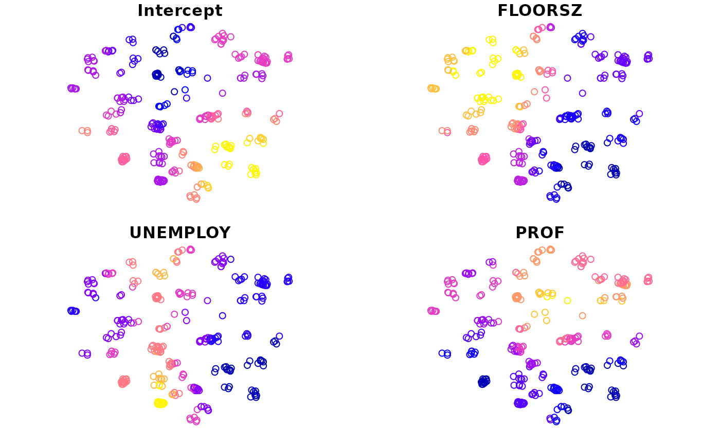
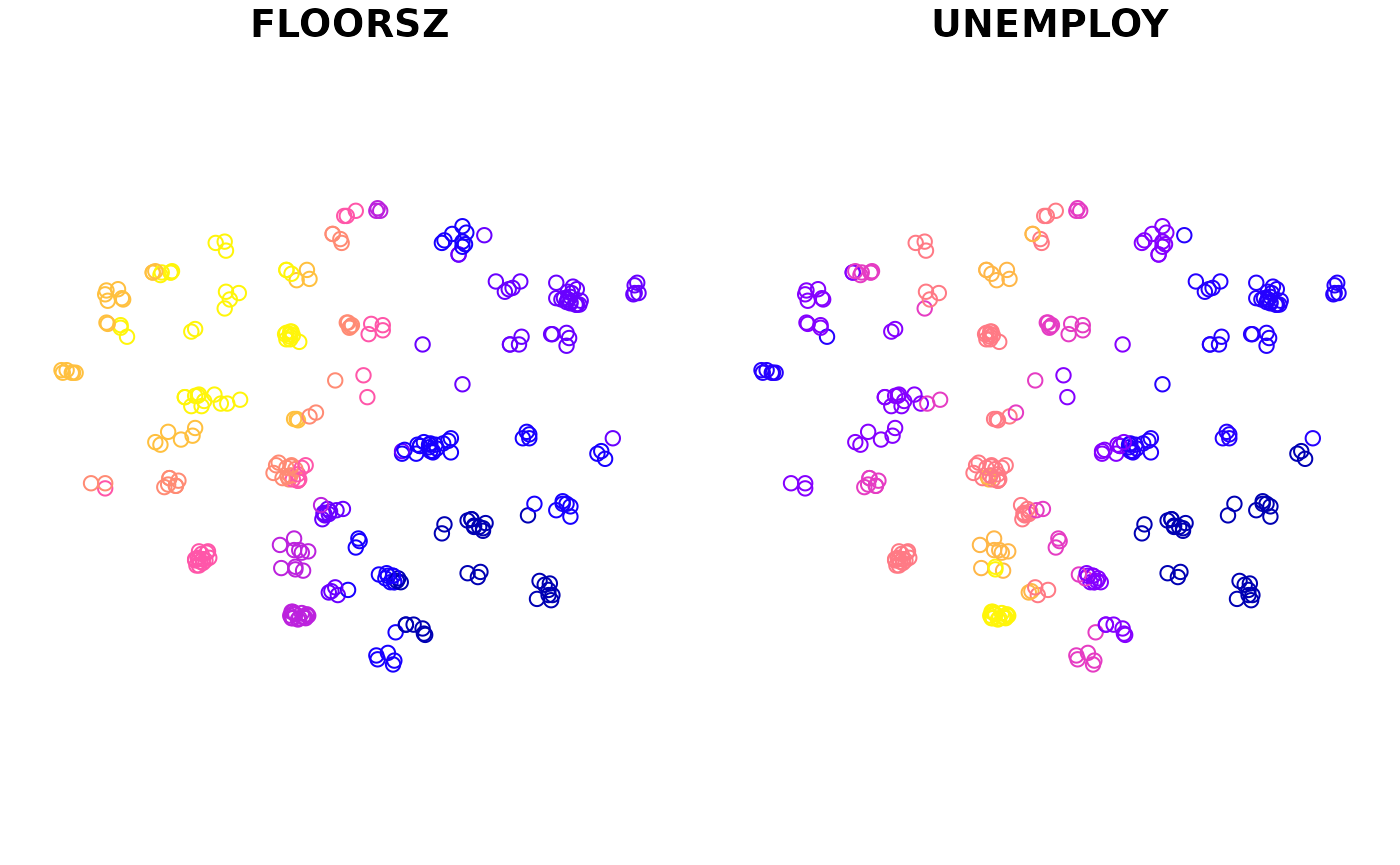
If the second argument is omitted, all coefficient estimates will be mapped by default. Otherwise, only specified variables will be mapped.
Weighting configurations
S4 class for dimension-specified weighting configrations
This package provides a S4 class named GWDRConfig, which is used to set dimension-specified weighting configurations. This class contains the following slots:
| Slot | Type | Descirption |
|---|---|---|
bw |
Numeric | Banwdith size. |
adaptive |
Logical | Whether the bandwidth is adaptive. |
kernel |
Character | Name of the kernel function. |
We can use the function gwdr_config() to create an object.
gwdr_config(0.618, TRUE, "bisquare")
#> An object of class "GWDRConfig"
#> Slot "bw":
#> [1] 0.618
#>
#> Slot "adaptive":
#> [1] TRUE
#>
#> Slot "kernel":
#> [1] "bisquare"
Replicating via rep() is enabled, but only the times parameter is supported.
rep(gwdr_config(36, TRUE, "bisquare"), 2)
#> [[1]]
#> An object of class "GWDRConfig"
#> Slot "bw":
#> [1] 36
#>
#> Slot "adaptive":
#> [1] TRUE
#>
#> Slot "kernel":
#> [1] "bisquare"
#>
#>
#> [[2]]
#> An object of class "GWDRConfig"
#> Slot "bw":
#> [1] 36
#>
#> Slot "adaptive":
#> [1] TRUE
#>
#> Slot "kernel":
#> [1] "bisquare"
Use GWDRConfig to configure arguments
The function gwdr() can not only set a uniform configuration, but also set each a configuration for dimensions.
Uniform configuration
To set a uniform configuration for all dimensions, just pass a list of only one GWDRConfig object. For example, the following code will set the bandwidth size to 10% samples for all dimensions.
m2 <- gwdr(
 formula = PURCHASE ~ FLOORSZ + UNEMPLOY + PROF,
 data = LondonHP,
 config = list(gwdr_config(0.2))
)
m2
#> Geographically Weighted Density Regression Model
#> ================================================
#>   Formula: PURCHASE ~ FLOORSZ + UNEMPLOY + PROF
#>      Data: LondonHP
#> Dimension-specified Weighting Configuration
#> -------------------------------------------
#>      bw unit   kernel
#> X 0.200    % gaussian
#> Y 0.200    % gaussian
#>
#>
#> Summary of Coefficient Estimates
#> --------------------------------
#>  Coefficient          Min.      1st Qu.       Median     3rd Qu.         Max.
#>    Intercept   -376593.420  -186375.440  -102639.928  -40136.756   137723.988
#>      FLOORSZ       901.315     1087.524     1522.518    1814.121     2840.217
#>     UNEMPLOY  -1317745.171    41504.759   435909.050  901915.439  2879552.062
#>         PROF   -127720.501   164473.936   249050.551  342561.859   540884.522
#>
#>
#> Diagnostic Information
#> ----------------------
#>   RSS: 272604534599
#>   ENP: 61.61364
#>   EDF: 254.3864
#>    R2: 0.8477754
#> R2adj: 0.8107603
#>   AIC: 7445.853
#>  AICc: 7512.849
Likewise, we can use the rep() function, but remember to use a right times argument, which should be equal to the number of independent variables (including the intercept if it exists).
m2 <- gwdr(
 formula = PURCHASE ~ FLOORSZ + UNEMPLOY + PROF,
 data = LondonHP,
 config = rep(gwdr_config(0.2), times = 2)
)
Separate configuration
To set configurations separately for each dimension, we need to input a list of GWDRConfig objects with the same number of elements to that of dimensions.
m3 <- gwdr(
 formula = PURCHASE ~ FLOORSZ + UNEMPLOY + PROF,
 data = LondonHP,
 config = list(gwdr_config(bw = 0.5, kernel = "bisquare"),
               gwdr_config(bw = 0.5, kernel = "bisquare"))
)
m3
#> Geographically Weighted Density Regression Model
#> ================================================
#>   Formula: PURCHASE ~ FLOORSZ + UNEMPLOY + PROF
#>      Data: LondonHP
#> Dimension-specified Weighting Configuration
#> -------------------------------------------
#>      bw unit   kernel
#> X 0.500    % bisquare
#> Y 0.500    % bisquare
#>
#>
#> Summary of Coefficient Estimates
#> --------------------------------
#>  Coefficient          Min.      1st Qu.       Median      3rd Qu.         Max.
#>    Intercept   -338426.177  -197024.579  -108199.954   -21037.803   208405.791
#>      FLOORSZ       874.665     1072.247     1441.932     1985.522     2578.291
#>     UNEMPLOY  -1684702.891    69860.819   502047.559  1278249.674  2274323.253
#>         PROF   -239863.434   149223.990   261570.242   368237.155   667653.133
#>
#>
#> Diagnostic Information
#> ----------------------
#>   RSS: 300737152296
#>   ENP: 50.34853
#>   EDF: 265.6515
#>    R2: 0.8320659
#> R2adj: 0.8001173
#>   AIC: 7469.247
#>  AICc: 7523.108
Then the functions c() rep() can be used to flexiably create such a list.
Bandwidth Optimization
The bandwidth optimization algorithm for GWDR requires a set of initial values for each parameter. Thus, even bandwidth optimization is enabled, it is necessary to set the initial values via the config argument. We can enable bandwidth optimization with the following codes.
m4 <- gwdr(
    formula = PURCHASE ~ FLOORSZ + UNEMPLOY + PROF,
    data = LondonHP,
    optim_bw = "AIC"
)
The method for optimizing bandwidth is specified through strings "AIC" or "CV". If the initial values are not appropriate, the function will use the default initial values instead: 61.8% samples for adaptive bandwidth, while 61.8% of maximum distance between samples for fixed bandwidth.
Model Selection
Apply the step() function to gwdrm objects to select the best model. Since version 4.1 of R, the pipe operator |> is avaliable. We can use the following code to enable model selection.
m5 <- gwdr(
    formula = PURCHASE ~ FLOORSZ + UNEMPLOY + PROF,
    data = LondonHP,
    optim_bw = "AIC"
) |> step(criterion = "AIC", threshold = 3, optim_bw = "AIC")
Where argument threshold is the threshold showing minimum changes of the criterion. Currently, only AIC criterion is supported, so the criterion here can only be "AIC".
For R of lower version, please use the following form:
m5 <- gwdr(
    PURCHASE ~ FLOORSZ + UNEMPLOY + PROF + BATH2 + BEDS2,
    LondonHP, optim_bw = "AIC"
)
m5 <- step(m5, criterion = "AIC", threshold = 10, optim_bw = "AIC")
m5
#> Geographically Weighted Density Regression Model
#> ================================================
#>   Formula: PURCHASE ~ FLOORSZ + PROF + UNEMPLOY
#>      Data: LondonHP
#> Dimension-specified Weighting Configuration
#> -------------------------------------------
#>      bw unit   kernel
#> X 0.155    % gaussian
#> Y 0.196    % gaussian
#>
#>
#> Summary of Coefficient Estimates
#> --------------------------------
#>  Coefficient          Min.      1st Qu.      Median      3rd Qu.         Max.
#>    Intercept   -610710.092  -185729.218  -87371.104   -10904.357   252299.605
#>      FLOORSZ       846.945     1058.576    1475.677     1914.966     3486.379
#>         PROF   -324882.636    89042.360  197398.378   313394.073   913105.451
#>     UNEMPLOY  -1996220.111  -223025.550  255246.558  1313205.723  6641280.360
#>
#>
#> Diagnostic Information
#> ----------------------
#>   RSS: 209784782000
#>   ENP: 85.57122
#>   EDF: 230.4288
#>    R2: 0.8828544
#> R2adj: 0.8391621
#>   AIC: 7383.702
#>  AICc: 7492.59
We can set config in step() to overwrite the original configurations. If it is not set, configurations in the gwdrm object will be applied. Further, if optim_bw is sepcified, bandwidth will be optimized afther the model selection.
The returned object after model selection contains a $step variable, in which there are all model combinations and corresponding criterions. There are three functions to visualize it.
step_view_circle(m5$step, main = "Circle View")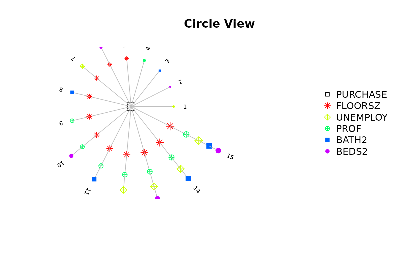
step_view_value(m5$step, main = "AIC Value")
step_view_diff(m5$step, main = "Diff of AIC")
They are:
- Variable combinations.
- Criterions for each combination.
- Difference of criterions. The improvement in the criterion for each combination compared with the previous one is clearly shown. This figure makes it easier to judge which model meets the requirement.
We can also use the universal plot() function which will make some modification to layouts.
plot(m5$step) # 等价于 step_view_circle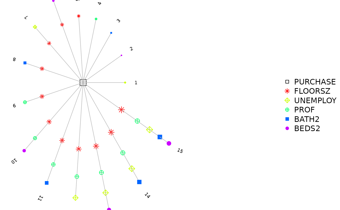
plot(m5$step, view = "value") # 等价于 step_view_value
plot(m5$step, view = "diff") # 等价于 step_view_diff
If further modification is required, use other arguments supported by plot().