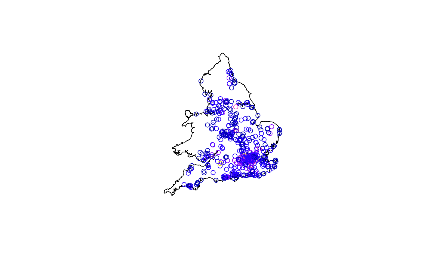
House price data set (DataFrame) in England and Wales

A house price data set for England and Wales from 2001 with 9 hedonic (explanatory) variables.

Usage

data(EWHP)

Format

A data frame with 519 observations on the following 12 variables.

Easting

a numeric vector, X coordinate

Northing

a numeric vector, Y coordinate

PurPrice

a numeric vector, the purchase price of the property

BldIntWr

a numeric vector, 1 if the property was built during the world war, 0 otherwise

BldPostW

a numeric vector, 1 if the property was built after the world war, 0 otherwise

Bld60s

a numeric vector, 1 if the property was built between 1960 and 1969, 0 otherwise

Bld70s

a numeric vector, 1 if the property was built between 1970 and 1979, 0 otherwise

Bld80s

a numeric vector, 1 if the property was built between 1980 and 1989, 0 otherwise

TypDetch

a numeric vector, 1 if the property is detached (i.e. it is a stand-alone house), 0 otherwise

TypSemiD

a numeric vector, 1 if the property is semi detached, 0 otherwise

TypFlat

a numeric vector, if the property is a flat (or 'apartment' in the USA), 0 otherwise

FlrArea

a numeric vector, floor area of the property in square metres

References

Fotheringham, A.S., Brunsdon, C., and Charlton, M.E. (2002), Geographically Weighted Regression: The Analysis of Spatially Varying Relationships, Chichester: Wiley.

Author

Binbin Lu binbinlu@whu.edu.cn

Examples

library(sf)
data(EWHP)
data(EWOutline)
ewhp_sf <- st_as_sf(EWHP, coords = c("Easting", "Northing"))
plot(EWOutline$geometry)
plot(ewhp_sf["PurPrice"], add = TRUE)